MATHS FOR ML

---

Scalar

Scalar is a physical quantity that is completely described by its magnitude.

Examples: Volume, speed, density etc.

---

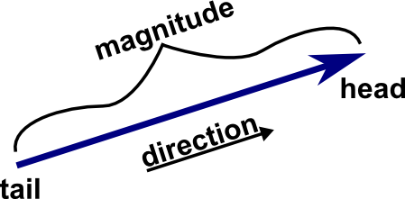
Vector

A vector is an object that has both a magnitude and a direction. Geometrically, we can picture a vector as a directed line segment, whose length is the magnitude of the vector and with an arrow indicating the direction.

Example: N-tuple $x\; =\; [x$₁, x₂,....x_N]

In Machine learning we call ordered list of feature value attributes as vector.

---

Set

A set in mathematics is a unordered collection of well defined and distinct objects.

Operations on set

• Union

  Two sets can be "added" together. The union of A and B, denoted by A ∪ B, is the set of all things which are members of either A or B.

  Example: $\{1,2,3\}\; \cup \; \{3,red,white\}\; =\; \{1,2,3,red,white\}$

• Intersection

  The intersection of A and B, denoted by A ∩ B, is the set of all things which are members of both A and B. If A ∩ B = ∅, then A and B are said to be disjoint.

  Example: $\{1,2,3\}\; \cap \; \{3,red,white\}\; =\; \{3\}.$

---

Some generl Notations

• Summation( ∑ ):

Example: The sum of a function F(x) from x=0 to n, will be written as $\sum$_x=0ⁿ F(x) .

• Multiplicaton( ∏):

  Example: The product of a function F(x) from x=0 to n, will be written as $\prod$_x=0ⁿ F(x).

• Defining a set:

  Example: S' ← {x³ ∣ x ∈ S, x > 5}

---

Vector Operations

$$

For vectors A=[a¹,a²,....aⁿ],B=[b¹,b²,....bⁿ] and scalar c.

• A + B = [a¹+b¹,a²+b²,....aⁿ+bⁿ]
• A - B = [a¹-b¹,a²-b²,....aⁿ-bⁿ]
• cA = [ca¹,ca²,....caⁿ]

---

Matrix Multiplication, Inverse and Transpose

A Matrix is an array of numbers:



This matrix has 2 Rows and 3 Columns, represented as 2×3 matrix.

• Multiplication

  Any two matrices of the form m×n and n×q can be multiplied, which results in a matrix of the form m×q.

  Example:

  

• Inverse

  The inverse of a matrix A is denoted by A^-1, such that A×A^-1 = I, where I is the identity matrix.

• Transpose

  The transpose of a matrix is a new matrix whose rows are the columns of the original. (This makes the columns of the new matrix the rows of the original).For example

  

---

Functions

A function f form a set X to Y is a mapping, such that each elemnt of X is mapped to a single element of Y.

For a function y=f(x)

• Local min/max

  f has a local minimum/maximum at a point c if f(x)≥f(c)/f(x)≤f(c) for every x in some open interval around c.

• Global Min/Max

  f has a global max if the function attains its maximum(similarly minimum value for min) in its whole domain.



• Max and Argument of Maxima

• Max_a∈Af(a)

  = Maximum value of f(a) for a∈A.

• ArgMax_a∈Af(a)

  = Argument of maxima is the element of set A at which f(a) is maximum.

---

Derivative

The derivative of y with respect to x is defined as the change in y over the change in x. In mathematical terms:

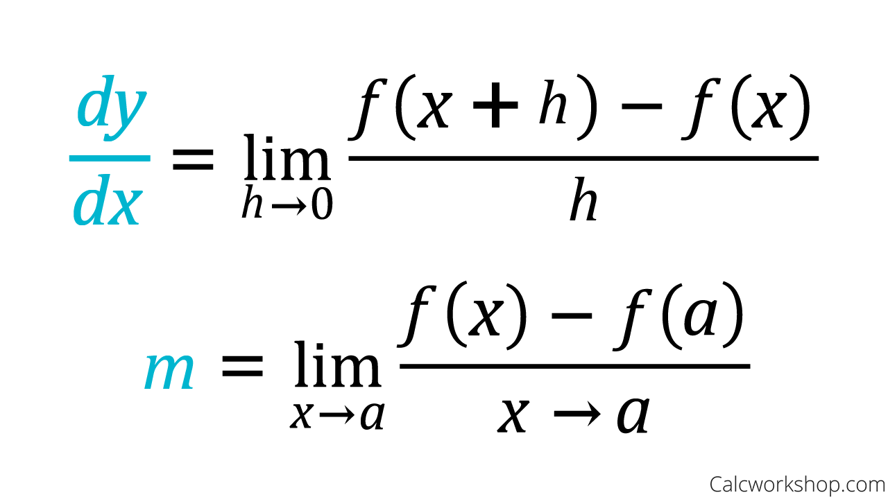
Differentiation is a method of finding the derivative of a function.

---

Gradient

For a funcion f:Rⁿ→Rⁿ, it's gradient ∇f:Rⁿ→Rⁿ is defined at the point p = (x₁,x₂,....x_n) in n-dimensional space as the vector-

Example: Let f(x,y) = x²y. Then ∇f = (2xy,x²). So ∇f(3,2) = (12,9) or 12i + 9j.

---

Random Variable

A random variable is described informally as a variable whose values depend on outcomes of a random phenomenon. There are two types of random variables, discrete and continuous.

• Discrete

  A discrete random variable is one which may take on only a countable number of distinct values. For example: If X represents the number of times that the coin comes up heads, then X is a discrete random variable that can only have the values 0,1,2,3. No other value is possible for X.

  The probability distribution of a discrete random variable is a list of probabilities associated with each of its possible values. It is also sometimes called the probability function or the probability mass function.

  Suppose a random variable X may take n different values, with the probability that X = x_i defined to be P(X = x_i) = p_i. The probabilities p_i for i=1 to n, must satisfy the following:

  • 0≤p_i≤1, for each i.
  • p₁ + p₂ +....+ p_n = 1

  For example: Lets consider a probability histohram:

  

  The variable X can take values 1,2,3,4. For each outcome, we have a probability,

  outcome	1	2	3	4
  Probability	0.1	0.3	0.4	0.2

  The probability that X is equal to 2 or 3 is the sum of the two probabilities: P(X=2 or X=3) = P(X=2) + P(X=3) = 0.3 + 0.4 = 0.7.

• Continuous

A continuous random variable is one which takes an infinite number of possible values. Continuous random variables are usually measurements. Examples include height, weight, the amount of sugar in an orange, the time required to run a mile.

A continuous random variable is not defined at specific values. Instead, it is defined over an interval of values, and is represented by the area under a curve. Probability density function(pdf) is a function that gives probabilty of a point.

For any continuous random variable with probability density function f(x), we have that:



For example:



The probability density fucnction(pdf) of this random variable looks like a bell shaed curve, and ∫ρ(x)dx = 1, where $\rho (x)\; =e-x2⁄2⁄\; \surd 2\pi$

• Expectation(E[x])

  The expected value of X, is a geeralization of the weighted average of the possible values that X can take, each value being weighted according to the probability of that event occurring.

  • For Discrete

    E[x] = ∑_i=1^k x_ip_i = x₁p₁ + x₂p₂ + ......+ x_kp_k

  • For Continuous

    E[x] = ∫xf(x)dx .