Linear Regression Model

Simple Linear Regression :

• A type of Supervised learning
• It uses different variables and parameters to produce a set of optimized parameters that can properly explain the relationship between variables.
• One of the most used algorithms for getting optimized parameters is Gradient Descent.

Gradient Descent

Gradient descent objective is to minimize the cost function, where cost function is defined as \begin{equation} J(m,c) = {1 \over n}\sum_{i=0}^{n}{(y_{i}(predicted)- y_{i}(actual))^2} \end{equation}
y(predicted) is also termed as hypothesis function for linear regression. $$ y(predicted) = mx + c$$ here x is the independent variable which we obtain through experiments and y is dependent variable which we obtain through two methods:

• Through the experiment (\(y_{i}(actual)\))
• Through the proposed model by obtaining optimized parameters (\(y_{i}(predicted)\))
Here m and c are the parameters that need to be optimized to \(m*,c*\) such that value of J gets minimized.
Just for convenience lets choose \(y_i(actual) \Rightarrow y_{i}^{a}\) and \(y_i(predicted) \Rightarrow y_{i}^{p}\).

How Gradient Descent Works ?

1. First we choose an initial parameter as \(m_0,c_0\)
$$y_{i}^{p} = m_{0} x_{i} + c_0$$
2. Now iteratively update m, b in such a way that J should decrease after each iteration:
$$ m = m - \alpha \Delta m $$ $$ c = c - \alpha \Delta c $$
where alpha is the learning parameter.
3. One needs to calculate \(\Delta m\) and \(\Delta c\), we define them in following way: $$ \Delta m = {\partial J(m,c) \over \partial m} $$ $$ \Delta c = {\partial J(m,c) \over \partial c} $$
4. We have defined the cost function as: $$J(m,c) = {1 \over n}\sum_{i=0}^{n}{(y_{i}^{p}- y_{i}^{a})^2}$$ Using the definition of \(y_{i}^{p} = m x_{i} + c \) $$ \Rightarrow J(m,c) = {1 \over n} \sum_{i=0}^{n}{(m x_{i} + c- y_{i}^{a})^2}$$ $$ {\partial J(m,c) \over \partial m} = {1 \over n} 2 \sum_{i=0}^{n}{(m x_{i} + c- y_{i}^{a}) m} $$ Similarly $$ {\partial J(m,c) \over \partial c} = {1 \over n} 2 \sum_{i=0}^{n}{(m x_{i} + c- y_{i}^{a}) c}$$ Now we subtitute these values in Step(2) and iterate until we get the best fit.

Learning parameter

In Step(2) we have mentioned something as Learning Parameter. It is quite crucial to know about this parameter, as its name suggests it is the learning parameter. It decides the rate of learning of the algorithm. The partial derivatives of J(w.r.t m or c) gives us the values of \(\Delta\)m, \(\Delta\)c such that J gets decreased. The iterative steps are taken in such a way in gradient descent that we attain the minima. This step size is determined by parameter \({\alpha}\). Conditions on \({\alpha}\):
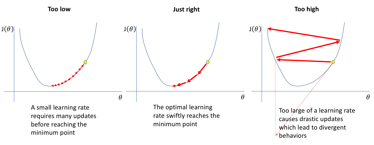in above image the \(\theta\) is parameter like m,c.

• If \(\alpha\) is too low: then it may result that we may take a lot of time to attain the minima of J(m,c) as th steps are too small.
• Optimum value of \(\alpha\): Generally it is around 0.001 to 0.1 but can vary for different datsets.
• If \(\alpha\) is too high: then it may result that we may not attain the minima of J(m,c) as th steps are too large.

Where can Gradient Descent work ?

• If the closed form solution doesnot exist then Gradient Descent would be one of the best algorithms for regression model.
• When the exact form solution is available, why would anyone need to use gradinet descent. There are other algorithms like Normal Equation method(2008 Normal Equations. In: The Concise Encyclopedia of Statistics. Springer, New York, NY.) that can easily work.
  But the problem with normal equations is, it requires a lot of computation as it involves the K*K dimensional matrices and it also requires inversion of those matrices. This increases cost of computation and time. Here gradient descent would be able to work easily than Normal Equation method.

Try Gradient Descent technique through this link by randomly giving points and observe the changes in line.

Reference

1. 2008 Normal Equations. In: The Concise Encyclopedia of Statistics. Springer, New York, NY.
2. Learning Parameter \(\alpha\)
3. Gradient Descent