Linear regression with multiple features
Introduction
In simple linear regression we have only one \(x\) (input feature) and one \(y\) (target variable). When we fit our data we'll get a line with the least sum of squared residuals. In linear regression with multiple variables, instead of a single input feature, we use multiple input features (assuming that it would help to make the prediction better). Here, when we fit our data, we would get a plane or a higher dimensional object(hyper-plane), depending on the number of input features we use.
Model
We assume \(y\) (target variable) as a linear function of \(x\) (input features) $${{f(x)=\sum_{i=0}^{n} w_{i} x_{i}}}$$
where n is the number of input features. f(x) depends on both, the parameters(w) and features(x) .
We fix \(x_{0}=1\), so that \(w_{0}\) is the intercept term. If we have 'n' input features, then \(W\) and \(X\) are (n+1) dimensional vectors, beacause we add an extra \(x_{0}\) and \(w_{0}\). Now for training data set, we need to pick the parameters. We will define a function, that measures, for each values of \(w\), how close the \(f_{w}\left(x^{(\imath)}\right)\) are to the corresponding \(y^{(i)}\). We define the cost function: $${{J(w)=\frac{1}{2} \sum_{i=1}^{m}\left(f_{w}\left(x^{(i)}\right)-y^{(i)}\right)^{2}}}$$
It is the least-square cost function that gives rise to the ordinary least squares regression model.
Our aim is to find value of w which reduces \(J(w)\) or the cost function.
Gradient Descent
We will optimize our cost function using Gradient Descent Algorithm.Here we find the value of \(w\) which reduces the cost fucntion. We will start with some \(W\) (which is an n+1 dimensional vector) and repeatedly changing \(W\) to reduce \(J(w)\), and in each iteration we update \(W\).
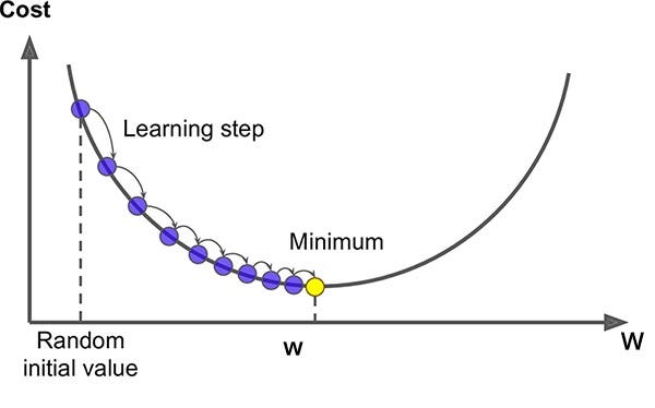
One step of gradient descent can be implemented as $${{w_{j}=w_{j}-\alpha \frac{\partial}{\partial w_{j}} J(w)}}$$ (= denotes the assignment of new value to \(w_{j}\)). This update is simultaneously performed for all values of j = 0, . . . , n, that is for all input features. Here \(\alpha\) is called the learning rate. The learning rate is a hyperparameter, which is the size of the each learning step.
Considering one training example: (x, y) $${{\begin{aligned} \frac{\partial}{\partial w_{j}} J(w) &=\frac{\partial}{\partial w_{j}} \frac{1}{2}\left(f_{w}(x)-y\right)^{2} \\ &=2 \cdot \frac{1}{2}\left(f_{w}(x)-y\right) \cdot \frac{\partial}{\partial w_{j}}\left(f_{w}(x)-y\right) \\ &=\left(f_{w}(x)-y\right) \cdot \frac{\partial}{\partial w_{j}}\left(\sum_{i=0}^{n} w_{i} x_{i}-y\right) \\ &=\left(f_{w}(x)-y\right) x_{j} \end{aligned}}}$$
So the new updated \(w_{j}\) for one training example is : $${{w_{j}:=w_{j}-\alpha\left(f_{w}\left(x^{(i)}\right)-y^{(i)}\right) x_{j}^{(i)}}}$$
for all the training example : $${{w_{j}:=w_{j}-\alpha\sum_{i=1}^{m}\left(f_{w}\left(x^{(i)}\right)-y^{(i)}\right) x_{j}^{(i)}}}$$ where \(x^{(i)}\) is the input feature of i th training example and \(y^{(i)}\) is the target label of i th training example. So in each iteration of gradient descent, the \(w_{(j)}\) is updated for j = 0,1,....,n, which are the number of input features.
Here we can see that, the magnitude of the update is proportional to the error term \(\left(f_{w}\left(x^{(i)}\right)-y^{(i)}\right)\); which means if the difference between predicted y and actual y is less, then the parameters have to changed in lesser extend only, but if the diference between predicted y and actual y is huge, that is, a large error, then there is need for lager change in paramteres.
Generally gradient decent is susceptible to local minima, however, here the cost function, J is a convex quadratic function, so, there is only one global, and no other local, optima; thus gradient descent always converges (assuming the learning rate \(\alpha\) is not too large).

Implementation
Let's first implement in python from scratch, which will help understand the theory a bit clearer. And after that we can use scikit-learn approach.
import seaborn as sns
import numpy as np
import pandas as pd
import matplotlib.pyplot as plt
plt.rcParams['figure.figsize'] =(11.7,8.27)
# Reading Data
data = pd.read_csv('electrical.csv')
print(data.shape)
data.head()
       Capital 	Labour 	Energy 	Electrical
0 	98.288 	0.386 	13.219 	1.270
1 	255.068 1.179 	49.145 	4.597
2 	208.904 0.532 	18.005 	1.985
3 	528.864 1.836 	75.639 	9.897
4 	307.419 1.136 	52.234 	5.907
capital = data['Capital'].values
labour= data['Labour'].values
energy = data['Energy'].values
electrical = data['Electrical'].values
#X matrix
m = len(capital)
x0 = np.ones(m)
X = np.array([x0, capital, labour, energy]).T
X.shape
#setting initial parameters as zeroes
W = np.array([0,0,0,0])
Y = np.array(electrical)
#f = np.dot(X,W)
#err = f-Y,error
#err_sq = (f-Y)**2, squared error
#init_error = np.sum(err_sq)/2
#X-dim-(1000,3),W-dim-(1,3), Y-dim-(1000,1)
#defining cost function

def cost_fn(X,W,Y):
    m = len(Y)
    J = np.sum((X.dot(W)-Y)**2)/(2*m)
    return J
inital_cost = cost_fn(X, W, Y)
print(inital_cost)
17.26223753125
#defining gradient decent algorithm to minimize the cost
def gradient_descent(X, Y, W, alpha, iterations):
    #cost_history appends the cost to itself after every iteration
    #updated_W appends the theta to itself after every iteration

    cost_history = list()
    updated_W = list()


    m = len(Y)

    for iteration in range(iterations):
        # predicted y values.
        f = X.dot(W)

        # Difference b/w predicted y values and actual Y
        loss = f - Y

        # Calculating the gradient
        gradient = X.T.dot(loss) / m

        # updating W using Gradient
        W = W - alpha * gradient
        updated_W.append(W)

        # New Cost
        cost = cost_fn(X, W, Y)
        cost_history.append(cost)


    return updated_W, cost_history
alpha = 0.00001 #learning rate
updated_W, cost_history = gradient_descent(X, Y, W, alpha, 120)

# New Values of theta, shows the latest value appended to the list
print('new_W:', updated_W[-1])

# Final Cost of new B, shows the latest value appended to the list
print('reduced_cost:',cost_history[-1])
new_W: [2.10368864e-04 1.15020092e-02 2.20620879e-05 1.36041074e-02]
reduced_cost: 0.8128226254518108
# Model Evaluation - RMSE
def rmse(Y, Y_pred):
    rmse = np.sqrt(sum((Y - Y_pred) ** 2) / len(Y))
    return rmse

# Model Evaluation - R2 Score
def r2_score(Y, Y_pred):
    mean_y = np.mean(Y)
    ss_tot = sum((Y - mean_y) ** 2)
    ss_res = sum((Y - Y_pred) ** 2) #sum of squared residuals
    r2 = 1 - (ss_res / ss_tot)
    return r2


Y_pred = X.dot(updated_W[-1])

print('rmse:', rmse(Y, Y_pred))
print('r2_score:', r2_score(Y, Y_pred))
rmse: 1.2750079415060995
r2_score: 0.8402052663759609
x = np.arange(1,len(cost_history)+1) #iterations
plt.plot(x,cost_history, linestyle='-', marker='o')
plt.xlabel("ITERATIONS")
plt.ylabel("COST J")
plt.show()

Implementation using scikit-learn
import seaborn as sns
import numpy as np
import pandas as pd
import matplotlib.pyplot as plt
plt.rcParams['figure.figsize'] =(11.7,8.27)
# Reading Data
data = pd.read_csv('electrical.csv')
print(data.shape)
data.head()
       Capital 	Labour 	Energy 	Electrical
0 	98.288 	0.386 	13.219 	1.270
1 	255.068 1.179 	49.145 	4.597
2 	208.904 0.532 	18.005 	1.985
3 	528.864 1.836 	75.639 	9.897
4 	307.419 1.136 	52.234 	5.907
capital= data['Capital'].values
labour= data['Labour'].values
energy = data['Energy'].values
electrical = data['Electrical'].values
from sklearn.linear_model import LinearRegression
from sklearn.metrics import mean_squared_error

# X and Y Values
X = np.array([capital,labour,energy]).T
Y = np.array(electrical)

# Model Intialization
model = LinearRegression()
# Data Fitting
model= model.fit(X, Y)
# Y Prediction
Y_pred = model.predict(X)

# Model Evaluation
rmse = np.sqrt(mean_squared_error(Y, Y_pred))
r2 = model.score(X, Y) #r2 is the square of correlation coefficient


print('rmse:',rmse)
print('r2 ',r2)
print('model coefficient: ', model.coef_)
print('model intercept: ', model.intercept_)
model coefficient:  [ 0.0022478  -0.59955627  0.09069419]
model intercept:  0.6371381814320403
F = np.column_stack(((capital, labour, energy))) #making a 16x3 numpy array stacking the 3 columns
S = np.dot(F,model.coef_)
S = S + model.intercept_ #adding the intercept value
print(S)
[ 1.82552732  4.96076807  2.4206967   7.585149    5.38437771  1.11614805
  3.92553325  3.21398151  0.76968898  9.77712918  7.78980092  2.46495346
 11.73325897  4.31734975  7.42040215  4.25023497]
plt.scatter(S,Y)
plt.plot(S,Y_pred, 'r')
plt.xlabel("linear combination of feature vectors")
plt.ylabel("actual y")
plt.show

References
- CS229, Stanford University
- StatQuest with Josh Starmer https://www.youtube.com/watch?v=zITIFTsivN8.
- Machine Learning by Tom Mitchell